Assessing differences in interactions between peaks
This workflow demonstrates how to use AQuA-tools with AQuA normalized samples in your local environment. Using locally installed AQuA-tools requires specific sample file formatting and parameter use, which are outlined below. For example purposes, this recipe can also be run in Docker and Tinker environments, but it is designed to show how you can work with your own samples not provided in remote environments. For recipes designed for use in Docker or Tinker environments, we recommend starting with Recipe_01: Calling loops from a sample.
This recipe will help you:
- Prepare local input files
- Define and organize the necessary variables
- Run a full workflow step by step
- Interpret the biological outcome
We will use the following AQuA-tools:
Motivation
With the assumption that relevant 2D interactions observed in a contact matrix (HiChIP) stem from 1D peaks (ChIP-seq), the value at the matrix bin (pixel) emanating from any two given peaks represents its contact frequency in nuclear space. Therefore, by ‘casting a net’ on the contact matrix using the combinatorics of all possible peaks within a given TAD, we get the entire interaction space between peaks of interest for a given sample. This interaction space can then be compared across conditions to ask: “is there a global observable difference in interaction counts between the interaction spaces of peaks between treatment and control?”
In this recipe, we’ll use two experimental conditions:
Case: H3K27ac HiChIP performed on the cell-line RH4 (DMSO)
Control: H3K27ac HiChIP performed on the cell-line RH4 treated with entinostat, an HDAC inhibitor.
For both experiments, we have paired linear 1D peaks from H3K27ac ChIP-seq experiments.
Chapter 0: Ingredients
I. Prerequisites
You must complete the AQuA-tools local installation before starting, which can be found here.
Installing locally will create the following structure in your home directory:
$HOME/├── aqua_tools/ # AQuA tools├── lab-data/ # Sample data├── outputs/ # To store output├── genome-wide_loops/ # Sample loops files├── bed_files/ # Sample peaks files├── juicer_tools_1.19.02.jar # Needed for plot_APANOTE: to know your $HOME path, simply type: echo $HOME
II. Format sample .hic data and .mergeStats.txt files
Running AQuA-tools locally requires a specific folder and filename structure, described here. We’ll format sample data to match those requirements for illustration purposes here. To use your own samples, use your sample paths and make sure your .hic and .txt files meet the formatting requirements.
# -----------------------------------------------------------------------------# Running AQuA-tools locally requires a specific sample folder and filename# structure. This example formats provided sample data to match those requirements.# If using your own samples, provide your own paths and ensure that your .hic and# .mergeStats.txt files match the expected naming and folder layout:##   ~/SAMPLE/#       ├── SAMPLE.hic#       └── SAMPLE.mergeStats.txt## -----------------------------------------------------------------------------# Each sample folder must include a .hic file and a .mergeStats.txt file.## A minimal .mergeStats.txt file must contain at least this row:#     valid_interaction_rmdup    [human_count]## If a second reads column is present, AQuA-tools will use AQuA normalization.# Otherwise, it will default to CPM normalization.##     valid_interaction_rmdup    [human_count] [mouse_count]# -----------------------------------------------------------------------------## Even when running this tutorial in Docker, this formatting step is required# because we'll be using the `--sample1_dir` argument with `query_bedpe`, which# expects a full path to a sample folder. The `--sample1_dir` argument allows# you to use your own local data by pointing to a folder that follows the# expected structure.## --------------------------# Sample 1: RH4 DMSO H3K27ac# --------------------------
# Provide full path to sample1's foldersample1=$HOME/lab-data/hg38/RH4_DMSO_H3K27ac/RH4_DMSO_H3K27ac_version_1
# Rename the .hic file to follow required format: SAMPLE/SAMPLE.hicmv "$sample1/RH4_DMSO_H3K27ac_version_1.allValidPairs.hic" \   "$sample1/RH4_DMSO_H3K27ac_version_1.hic"
# Rename mergeStats.txt to match sample namemv "$sample1/mergeStats.txt" \   "$sample1/RH4_DMSO_H3K27ac_version_1.mergeStats.txt"
# --------------------------# Sample 2: RH4 HDACi H3K27ac# --------------------------
# Provide full path to sample2's foldersample2=$HOME/lab-data/hg38/RH4_HDACi_H3K27ac/RH4_HDACi_H3K27ac_version_1
# Rename the .hic file to follow required format: SAMPLE/SAMPLE.hicmv "$sample2/RH4_HDACi_H3K27ac_version_1.allValidPairs.hic" \   "$sample2/RH4_HDACi_H3K27ac_version_1.hic"
# Rename mergeStats.txt to match sample namemv "$sample2/mergeStats.txt" \   "$sample2/RH4_HDACi_H3K27ac_version_1.mergeStats.txt"
III. Gathering necessary files
For this workflow, we will need H3K27ac peaks files (.bed), a reference TAD file (.bed), a reference CTCF file (.bed from ENCODE-3 cCRE) and a TSS annotation file (.bed from GENCODE). We will assign these files to variable names for simpler use.
NOTE: we are using reference TAD and CTCF annotations for this recipe, as HiC-informed TAD calls and ChIP-informed CTCF peaks are lacking.
# Initialise files in variablesDMSO_peaks=$HOME/bed_files/RH4_DMSO_H3K27ac-peaks_GSM3229491_hg38.bed
HDACi_peaks=$HOME/bed_files/RH4_HDACi_H3K27ac-peaks_GSM3229493_hg38.bed
TSS=$HOME/lab-data/hg38/reference/GENCODE_TSSs_hg38.bed
CTCF=$HOME/lab-data/hg38/reference/ENCODE3_cCRE-CTCF_hg38.bed
TAD=$HOME/lab-data/hg38/reference/TAD_goldsorted_span_centromeres-removed_hg38.bed
Chapter 1: Building interaction spaces
I. Building the .bedpe
The AQuA tool build_bedpe can create the scaffold for assessing the combinatorial space of all possible 2D interactions using .bed files. The resulting output is a .bedpe file, which can be then used to query values from a contact matrix. The total set of possible interactions from a build_bedpe self-build is represented in Figure 1. For more information about how build_bedpe works, see our Docs.
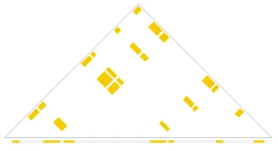
Fig 1. All possible interactions resulting from a build_bedpe self-build. Bed elements are depicted along the diagonal and interactions are shown in the triangle.
In this example, we’ll create two self-interaction .bedpe files, one for each condition (DMSO and HDACi), using their respective peak files. We set a minimum distance of 25kb between interaction anchors to avoid short-range contacts near the diagonal, and we restrict interactions to occur within TADs. This setup gives us the best chance of capturing interactions anchored in open chromatin with minimal noise from short-range contacts.
cd $HOME
build_bedpe \ --bed_A $DMSO_peaks \ --bed_B $DMSO_peaks \ --min_dist 25000    \ --TAD $TAD  > $HOME/outputs/RH4_DMSO_peaks.bedpe
build_bedpe \ --bed_A $HDACi_peaks \ --bed_B $HDACi_peaks \ --min_dist 25000     \ --TAD $TAD  > $HOME/outputs/RH4_HDACi_peaks.bedpe
Chapter 2: Constraining interaction spaces
I. Intersecting .bedpe with a TSS file
We can then reduce this combinatorial space of interacting peaks to interactions that have at least one TSS on either end of a .bedpe row using intersect_bedpe. This narrows our combinatorial scaffold of interactions to contain genes found in open chromatin and possibly poised for transcription. For more information about how intersect_bedpe works, see our Docs.
intersect_bedpe \ --bed_A $TSS \ --bedpe $HOME/outputs/RH4_DMSO_peaks.bedpe \    > $HOME/outputs/RH4_DMSO_peaks-tss.bedpe
intersect_bedpe \ --bed_A $TSS \ --bedpe $HOME/outputs/RH4_HDACi_peaks.bedpe \    > $HOME/outputs/RH4_HDACi_peaks-tss.bedpe
II. Intersecting .bedpe with a CTCF file
We’ll use intersect_bedpe again, this time with a .bed file containing reference CTCF sites obtained from ENCODE-3. By intersecting with CTCF sites, we narrow our focus to interactions mediated or stabilized by CTCF among regions already anchored at transcription start sites. This gives us a focused set of promoter-associated loops to continue our analysis with.
intersect_bedpe \ --bed_A $CTCF \ --bedpe $HOME/outputs/RH4_HDACi_peaks-tss.bedpe \    > $HOME/outputs/RH4_DMSO_peaks-tss-ctcf.bedpe
intersect_bedpe \ --bed_A $CTCF \ --bedpe $HOME/outputs/RH4_HDACi_peaks-tss.bedpe \    > $HOME/outputs/RH4_HDACi_peaks-tss-ctcf.bedpe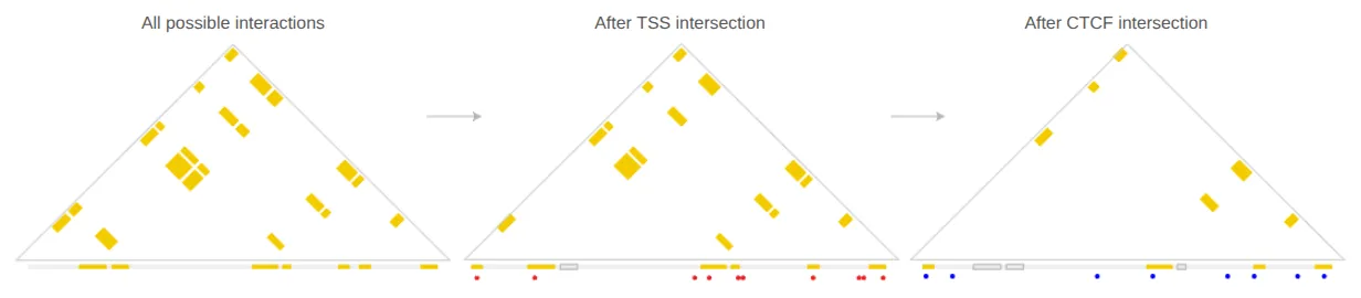
Fig 2. Reduction in interactions resulting from intersect_bedpe. Starting with the full set of interactions obtained from a self-build build_bedpe call, interactions are restricted to those that intersect with a TSS, and then restricted again to those that intersect with a CTCF site. TSSs are shown in red along the diagonal. CTCF sites are shown in blue along the diagonal. Filtered .bed elements are shown as gray boxes along the diagonal.
Chapter 3: Refining interaction spaces
I. Querying the .bedpe
The constrained set of interaction space obtained using steps above can then be paired with a contact matrix to query the respective interaction values for each row.
We will use query_bedpe with --formula max and --fix false to refine our input .bedpe coordinates. As the interaction space for any two given peaks can span multiple pixels in the contact matrix, choosing the max pixel hones into a single number with the most signal and keeps all .bedpe coordinates fixed to the resolution of choice (in this case the default of 5kb).
The refining process is visually represented in Figure 3. For more information about how query_bedpe works, see our Docs.
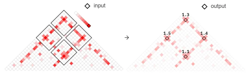
Fig 3. Refined interaction coordinates obtained from query_bedpe using --formula max and --fix FALSE.
For this step, we’ll be using our sample data folders which contain our .hic and .mergeStats.txt files.
NOTE: It’s important to use the --sample1_dir parameter when working with your own samples (or when following this recipe exactly for example purposes), rather than the --sample1 parameter, which is used in other recipes designed for use in Docker or Tinker environments.
query_bedpe \ --bedpe $HOME/outputs/RH4_DMSO_peaks-tss-ctcf.bedpe \ --sample1_dir $sample1 \ --formula max \ --fix FALSE > $HOME/outputs/RH4_DMSO_query.bedpe
query_bedpe \ --bedpe $HOME/outputs/RH4_HDACi_peaks-tss-ctcf.bedpe \ --sample1_dir $sample2 \ --formula max \ --fix FALSE > $HOME/outputs/RH4_HDACi_query.bedpe
Before continuing, let’s quickly check our output files to make sure we have bedpe coordinates in the first 6 columns and that we did not pick up any error messages.
head -n 2 "$HOME/outputs/RH4_DMSO_query.bedpe" | cut -f1-6
# chr10  102130000  102135000  chr10  102635000  102640000# chr10  103965000  103970000  chr10  104205000  104210000
head -n 2 "$HOME/outputs/RH4_HDACi_query.bedpe" | cut -f1-6
# chr10  102130000  102135000  chr10  102635000  102640000# chr10  103965000  103970000  chr10  104205000  104210000
Everything looks good here! Let’s move on to Chapter 4.
Chapter 4: Merging interaction spaces
I. Merging the .bedpe
So far, we have been working with each condition (DMSO and HDACi) separately, creating and refining the interaction spaces of each dataset.
Now, we will use union_bedpe to merge the spaces into a single .bedpe file. This step takes the union of overlapping interaction regions from the two conditions, creating a unified set of candidate loops for comparison. For more information about how union_bedpe works, see Figure 4 as well as our Docs.
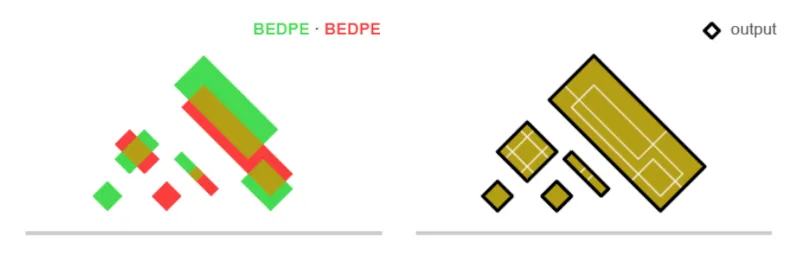
Fig 4. Merged interaction coordinates obtained from union_bedpe.
union_bedpe \ --bedpe $HOME/outputs/RH4_DMSO_query.bedpe \ --bedpe $HOME/outputs/RH4_HDACi_query.bedpe \ > $HOME/outputs/RH4_union.bedpeChapter 5: Visualizing interactions
I. Two-sample plot_APA with AQuA normalization
Finally, we can visualize the aggregate contact signal of the merged interaction space across the two conditions using plot_APA.
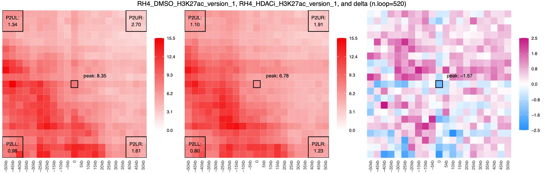
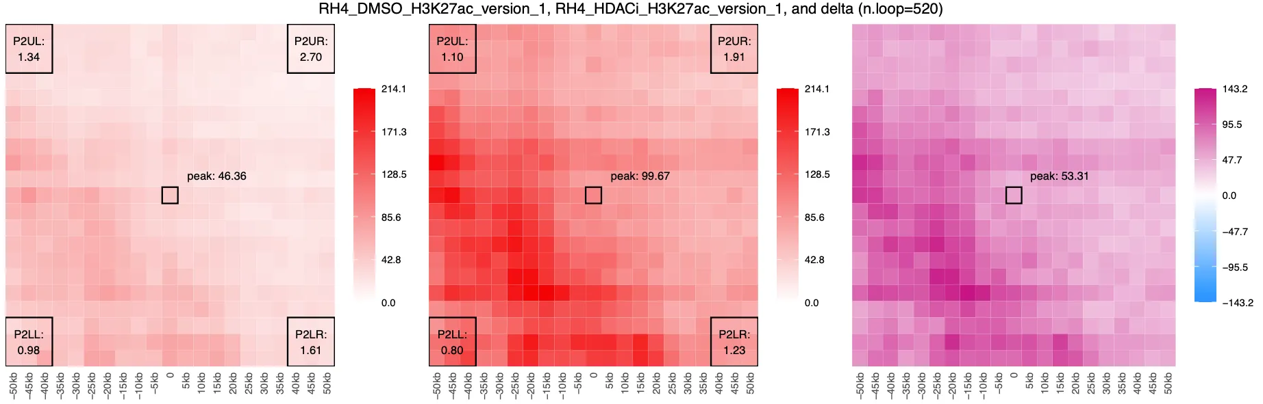
We’ll make a two-sample delta APA plot using both the RH4_DMSO and RH4_HDACi samples and our unified .bedpe. We’ll run plot_APA twice: once using CPM normalization and once using AQuA normalization. Because this dataset includes spike-in mouse reads, AQuA normalization is applied by default. For more information about how plot_APA works, see our Docs.
plot_APA \ --bedpe $HOME/outputs/RH4_union.bedpe \ --sample1_dir $sample1 \ --sample2_dir $sample2 \ --out-dir $HOME/outputs/RH4_aquaII. Two-sample plot_APA with CPM normalization
plot_APA \ --bedpe $HOME/outputs/RH4_union.bedpe \ --sample1_dir $sample1 \ --sample2_dir $sample2 \ --norm cpm \ --out-dir $HOME/outputs/RH4_cpmTo view the resulting APA plots, navigate to the output directories created for each plot and view the .pdf.
CPM output:
AQuA output:
Conclusion
In this recipe, we:
- Built the entire possible interaction space between linear H3K27ac peaks for each condition
- Constrained the interaction space to contain TSSs
- Further constrained the interaction space to contain CTCF sites
- Refined the coordinates of the interaction space to correspond to the maximum contact values
- Merged the interaction spaces across conditions
- Visualized the aggregate of the merged space in CPM and AQuA normalizations
Using CPM normalization, we observe lost interactions between peaks (centred ‘+’ blue) amongst a crackle of surrounding gains. However, when using AQuA, we observe a global overall gain in interactions. This pattern is consistent with findings from Gryder et al. 2020, who showed that AQuA normalization using an orthogonal spike-in can uncover global changes in chromatin interactions that CPM may miss. Specifically, AQuA reveals broad increases in H3K27ac-mediated looping after HDAC inhibition, which points to a shift in enhancer–promoter architecture beyond individual loops.
Why does that matter? Many biological processes depend not just on a handful of punctate loops, but on an overall loosening or tightening of the chromatin landscape. In other words, if you only focus on individual hotspots, you risk missing the forest for the trees: AQuA helps reveal when the entire forest is greening.
We designed the AQuA-tools suite to make it easy to take full advantage of the AQuA normalization method. AQuA-tools that use sample data automatically check the .mergeStats.txt file to determine whether spike-in reads are present. If spike-in data is found, AQuA normalization is applied by default. If not, the tools default to CPM normalization. Our hope is to simplify the process of analyzing your own samples, whether they include spike-in or not.
Once you’ve completed this recipe, we recommend exploring the next recipe designed for Tinker and Docker environments. There, you’ll be introduced to extract_bedpe, a powerful AQuA tool that uses inherent normalization to call loops directly from HiChIP contact matrices, with no peak file required. These next steps offer a novel and flexible approach to discovering chromatin interactions and are perfect for diving deeper into what AQuA-tools can do.
Gryder, B. E., Khan, J., & Stanton, B. Z. (2020). Measurement of differential chromatin interactions with absolute quantification of architecture (AQuA-HiChIP). Nature protocols, 15(3), 1209–1236. https://doi.org/10.1038/s41596-019-0285-9