Calling loops from a sample

This workflow demonstrates how to call loops using AQuA-tools in a Docker or Tinker environment.

We will use the following AQuA tools:

Motivation

In the previous recipe, we focused our analysis on HiChIP contacts between known linear 1D peaks derived from prior ChIP-seq data. However, very often we do not have paired ChIP experiments, and it becomes necessary to call meaningful interactions directly from the contact matrix itself. In such cases, obtaining a visually appealing set of loop calls is critical before performing any downstream operation for hypothesis testing.

In this recipe, we’ll use two independent cell lines:

sample1: H3K27ac HiChIP performed on the cell line GM12878
sample2: H3K27ac HiChIP performed on the cell line K562

For both experiments, we do not have paired linear 1D peaks from H3K27ac ChIP-seq experiments.

Chapter 0: Ingredients

I. Prerequisites

You must complete the AQuA-tools Docker installation before starting, which can be found here. Alternatively, if you have access to Tinker, AQuA-tools are already pre-installed and no installation is needed.

II. Creating a workspace

This is an optional step. We encourage users to organize their analyses into a directory structure that keeps things nice and clean.

working_directory=/home/ubuntu/container_outputs
mkdir -p $working_directory
cd $working_directory
mkdir -p \
 data \
 scripts \
 results \
 scratch

It’s nice to have all the files you want to play with in $working_directory/data

For now, we’ll follow the steps of this tutorial by housing ourselves in $working_directory/scratch, but we recommend writing .sh scripts in $working_directory/scripts and storing the results in $working_directory/results

III. Gathering necessary files

For downstream analysis, we will need a TAD file and a TSS file. We’ll assign these file paths to variable names for easier calling later.

cd $working_directory/scratch

# Initialise files in variables
TAD=/home/ubuntu/lab-data/hg38/reference/TAD_goldsorted_span_centromeres-removed_hg38.bed

TSS=/home/ubuntu/lab-data/hg38/reference/GENCODE_TSSs_hg38.bed

IV. Find a genomic region of interest

Now that we have our TAD and TSS files, we can choose a locus to use in our downstream analysis. For this recipe, we will use bedtools intersect to find the TAD that contains the MYC locus, but you can use this process for any gene of interest to you.

# Get coordinates for MYC locus from TSS file
# NOTE: all gene names are in upper case
grep -w MYC $TSS > MYC.bed
cat MYC.bed
# chr8  127735434  127735435  MYC  +

# Get coordinates of the TAD that contains MYC
bedtools intersect -a $TAD -b MYC.bed -wa -wb
# chr8  126817755  129115254  8  chr8  127735434  127735435  MYC  +

The first three columns are the range of the TAD where MYC resides, which we will use as the genomic range to tinker with when calling loops. When specifying a range to AQuA tools, the required format is chr:start:end

# Storing TAD coordinates in a variable
myc_tad=$(bedtools intersect -wa -a "$TAD" -b <(awk '$4=="MYC" {print}' "$TSS") | awk '{print $1 ":" $2 ":" $3}')

echo $myc_tad
# chr8:126817755:129115254

V. Defining a sample

We’ll need a sample to get started. In Tinker or Docker environments, you’ll use the name of the sample as it appears on the Tinker box or Docker container.

# on Tinker or Docker
sample=GM12878_H3K27ac

NOTE: You can list all loaded samples on your tinkerbox or Docker container using list_samples

Chapter 1: Calling loops for a region of interest

The loop-calling tool in the AQuA-tools suite is extract_bedpe. extract_bedpe scans all possible bin‐pairs within a defined region (or regions, think TADs), and outputs those .bedpe pairs with contact scores above a user‐defined inherent score and distance threshold. To know more about inherent scores, check out our Docs.

I. Extracting the `.bedpe`

In this example, we’ll use extract_bedpe to scan the sample and region defined in Chapter 0. This recipe covers several key features of the tool, but we also recommend checking out our Docs to learn more about how it works.

extract_bedpe \
 --sample1 $sample \
 --range $myc_tad  \
 --genome hg38     > GM12878_MYC.bedpe

II. Viewing the `.bedpe`

We can visualize the output of extract_bedpe with the AQuA-tool plot_contacts. This tool accepts a .bedpe file via the --bedpe parameter, which will highlight the regions in the .bedpe on the contact plot. For more information about how plot_contacts works, see our Docs.

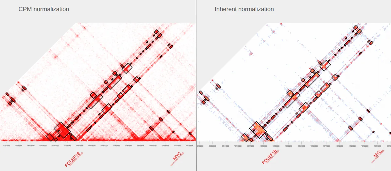
plot_contacts \
  --sample1 $sample  \
  --range $myc_tad   \
  --genome hg38      \
  --bedpe GM12878_MYC.bedpe \
  --output_name MYC.pdf

On Tinker, you can view this pdf by downloading it from the file browser. On Docker, you can open the file directly from your local output directory.

Here’s our pdf! plot1

Chapter 2: Changing extraction parameters

I. Changing the `extract_bedpe` threshold score

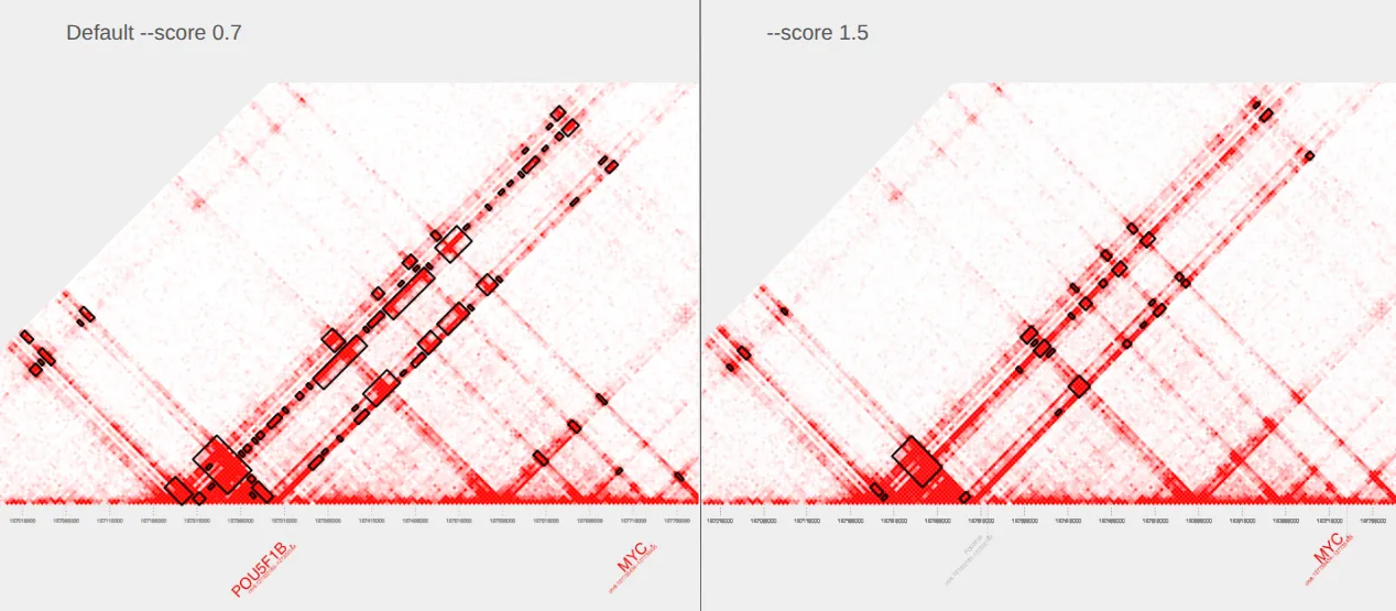
In this step, we’ll re-run the same extract_bedpe command from Chapter 1, but with an additional --score parameter to set a custom score threshold. This allows us to control which loops are extracted based on contact strength. Since extract_bedpe uses inherent normalization, most loop scores fall between 0 and 1. The default threshold is 0.7, but by increasing it to 1, we focus on loops with the strongest contact signals.

extract_bedpe \
 --sample1 $sample \
 --range $myc_tad  \
 --genome hg38     \
 --score 1         > GM12878_MYC_score-1.bedpe

We can view the output of extract_bedpe using plot_contacts once again:

plot_contacts \
  --sample1 $sample \
  --range $myc_tad  \
  --genome hg38     \
  --bedpe GM12878_MYC_score-1.bedpe \
  --output_name MYC_score-1.pdf

Here is the updated PDF! Notice that the highlighted .bedpe regions now align more closely with the strongest loop structures, appearing slightly smaller and more focused than in the previous plot.

plot2

II. Changing the `extract_bedpe` mode

—mode glob

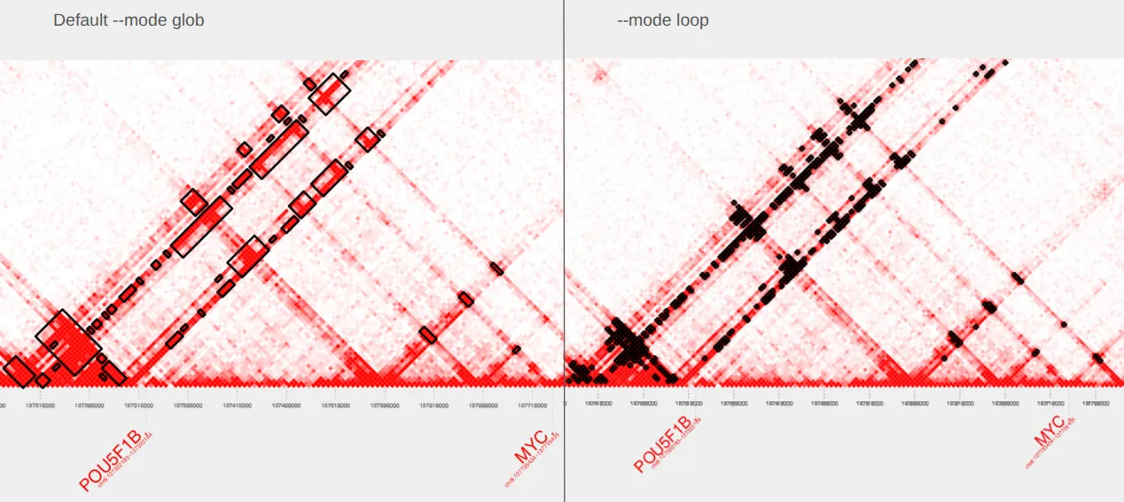
The default mode for extract_bedpe is --mode glob, which requires loops to span at least two consecutive bins. This helps eliminate loops that may be noise, and is the mode we have been using by default so far.

—mode loop

To view individual loops, we’ll use --mode loop with extract_bedpe and then plot with plot_contacts.

extract_bedpe \
 --sample1 $sample \
 --range $myc_tad  \
 --genome hg38     \
 --score 1         \
 --mode loop > GM12878_MYC_score-1_loop.bedpe


plot_contacts \
  --sample1 $sample \
  --range $myc_tad  \
  --genome hg38     \
  --bedpe GM12878_MYC_score-1_loop.bedpe \
  --output_name MYC_score-1_loop.pdf

Here is a zoomed in view of our extracted bedpe with --mode loop specified.

plot3

—mode flare

With --mode flare, extract_bedpe identifies clusters of bins above the --score threshold that flare outward from the diagonal and collapses each cluster into an elongated flare-shaped region.

extract_bedpe \
 --sample1 $sample \
 --range $myc_tad  \
 --genome hg38     \
 --score 1         \
 --mode flare > GM12878_MYC_score-1_flare.bedpe


plot_contacts \
  --sample1 $sample \
  --range $myc_tad  \
  --genome hg38     \
  --bedpe GM12878_MYC_score-1_flare.bedpe \
  --output_name MYC_score-1_flare.pdf

Here is a zoomed in view of our extracted bedpe with --mode flare specified.

plot4

—mode minimal

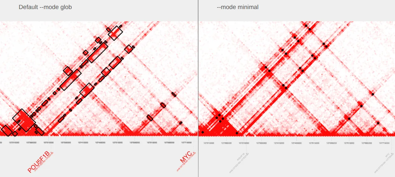
With --mode minimal, extract_bedpe detects the strongest interaction anchors based on both signal strength and interconnectivity. This produces a minimal loop set containing the most important features in the interaction network.

extract_bedpe \
 --sample1 $sample \
 --range $myc_tad  \
 --genome hg38     \
 --score 1         \
 --mode minimal > GM12878_MYC_score-1_minimal.bedpe


plot_contacts \
  --sample1 $sample \
  --range $myc_tad  \
  --genome hg38     \
  --bedpe GM12878_MYC_score-1_minimal.bedpe \
  --output_name MYC_score-1_minimal.pdf

Here is a zoomed in view of our extracted bedpe with --mode minimal specified.

plot5

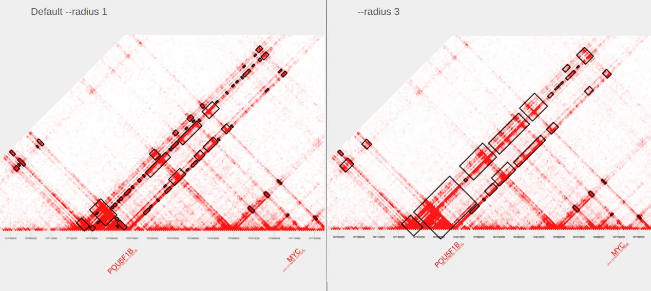
III. Changing the `extract_bedpe` radius

When using --mode glob or --mode flare, the --radius parameter determines the gap between reported regions of interaction. The default --radius is 1, but can be increased to join more distant bins. Here we compare .bedpe files made with the default --radius 1 and an increased --radius 3.

Default --radius 1:

plot6

With --radius 3:

extract_bedpe \
 --sample1 $sample \
 --range $myc_tad  \
 --genome hg38     \
 --radius 3 \
 --score 1         > GM12878_MYC_score-1_radius-3.bedpe


plot_contacts \
  --sample1 $sample \
  --range $myc_tad  \
  --genome hg38     \
  --bedpe GM12878_MYC_score-1_radius-3.bedpe \
  --output_name MYC_score-1_radius-3.pdf

plot7

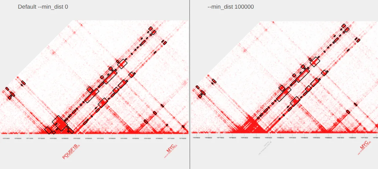
IV. Changing the `extract_bedpe` min_dist

To exclude loops close to the diagonal, we can supply a --min_dist value to extract_bedpe. Here, we filter pairs that are separated by less than 100,000 bp and plot.

extract_bedpe \
 --sample1 $sample \
 --range $myc_tad  \
 --genome hg38     \
 --score 1         \
 --mode loop       \
 --min_dist 100000 > GM12878_MYC_score-1_loop_mindist-100kb.bedpe


plot_contacts \
  --sample1 $sample \
  --range $myc_tad \
  --genome hg38 \
  --bedpe GM12878_MYC_score-1_loop_mindist-100kb.bedpe \
  --output_name MYC_score-1_loop_mindist-100kb.pdf

Notice the loss of loops nearest the diagonal compared to the previous --mode loop plot.

plot8

Chapter 3: Genome-wide Loop Calling

I. Extracting the genome-wide .bedpe

extract_bedpe can be used to call loops across the entire genome, although this process is slower than the examples in previous chapters using a defined range for a locus, like MYC. Calling loops genome-wide can take up to 30 minutes. If you’re working on Docker, you have access to pre-computed genome-wide loop files in the directory /home/ubuntu/genome-wide_loops and you can skip this step.

# Genome wide loop calling

extract_bedpe \
 --sample1 GM12878_H3K27ac \
 --genome hg38 \
 --TAD $TAD \
 --min_dist 20000 > GM12878_genome-wide-loops.bedpe

extract_bedpe \
 --sample1 K562_H3K27ac \
 --genome hg38 \
 --TAD $TAD \
 --min_dist 20000 > K562_genome-wide-loops.bedpe

We’ll be using the output from this step in the next recipe.

Conclusion

In this recipe, you learned how to call chromatin loops using extract_bedpe and visualize them with plot_contacts in a Docker or Tinker environment. Starting from a single genomic region, we walked through how to fine-tune loop calling parameters like score thresholds, modes, radius, and minimum distance.

This approach provides a way to explore HiChIP contact maps directly, without predefined annotations like enhancers, promoters, or TADs. Our goal is to make tailored loop calling easy for your biological question, whether you’re zooming in on a gene like MYC or scanning the entire genome for large-scale interaction patterns. What might extract_bedpe uncover in your data?

In the next recipe, we’ll build on the results from this recipe by integrating genome-wide loop calls into comparative analyses. But before moving on, feel free to experiment with other regions, scores, and visualization styles to get a feel for how AQuA-tools works with your data.