Visualizing Loops

This code snippet shows how to visualize loops with plot_contacts in a Docker or Tinker environment.

We’ll use the same sample we used to call loops in the previous snippet.

sample=GM12878_H3K27ac

We’ll also define the genome build and range of interest.

genome=hg38
range=chr2:64500000:65000000

Here we assign the path to our loops file to a variable:

loops=my_loops.bedpe

And let’s give a name for our output .pdf:

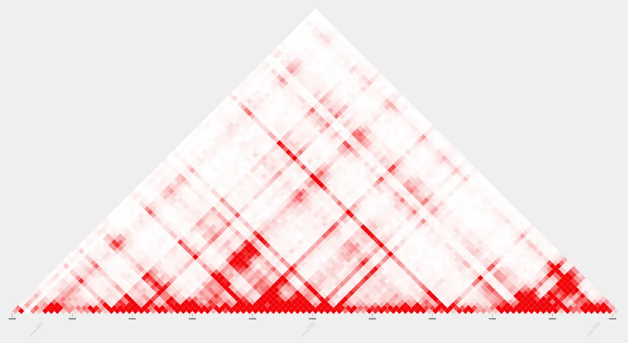
name=contact_plot.pdf

First, let’s run plot_contacts to look at our contact plot without our loops highlighted.

plot_contacts --sample1 $sample --genome $genome --range $range --output_name $name

Here’s our pdf:

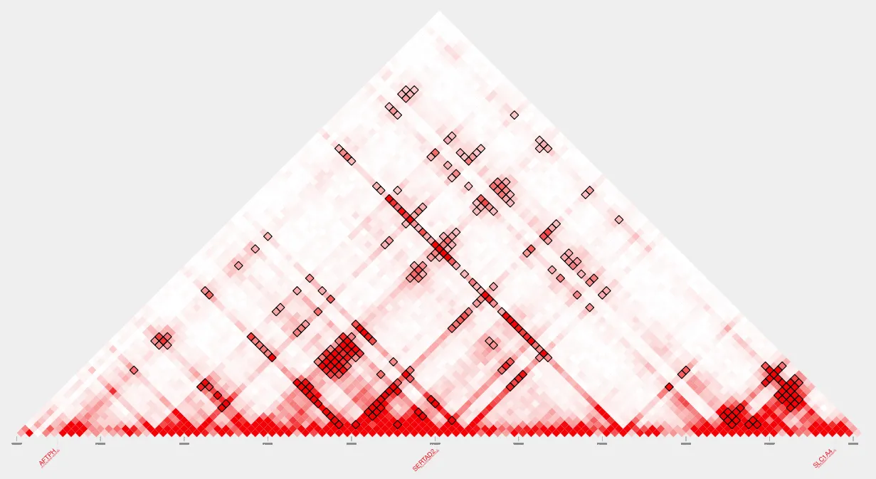
Next, let’s run the same code again with the addition of the --bedpe parameter to highlight our loops. We’ll also update the output name for this plot:

name=my_loops.pdf
plot_contacts --sample1 $sample --genome $genome --range $range --bedpe $loops --output_name $name

Here’s our pdf:

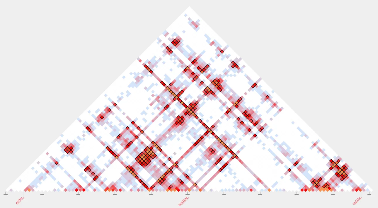
To apply Inherent Normalization, set the parameter --inherent to TRUE.

name=my_loops_inh.pdf
plot_contacts --sample1 $sample --genome $genome --range $range --bedpe $loops --output_name $name --inherent TRUE

Here’s our inherent normalized plot:

To intersect these loops with other regions of interest, please continue to the next Snippet: Intersecting Loops